3.1 - Building an Empty World
When we tell Player to build a world we only give it the .cfg file as an input. This .cfg file needs to tell us where to find our .world file, which is where all the items in the simulation are described. To explain how to build a Stage world containing nothing but walls we will use an example.
To start building an empty world we need a .cfg file. First create a
document called empty.cfg (i.e. open in your favorite text editor -
gedit is a good starter program if you don’t have a favorite) and
copy the following code into it:
driver
(
   name "stage"
   plugin "stageplugin"

   provides ["simulation:0" ]

   # load the named file into the simulator
   worldfile "empty.world"
)
The configuration file syntax is described in Chapter
4, but basically what is happening here is that your
configuration file is telling Player that there is a driver called
stage in the stageplugin library, and this will give Player data
which conforms to the simulation interface. To build the simulation
Player needs to look in the worldfile called empty.world which is
stored in the same folder as this .cfg. If it was stored elsewhere you
would have to include a filepath, for example ./worlds/empty.world.
Lines that begin with the hash symbol (#) are comments. When you build a
simulation, any simulation, in Stage the above chunk of code should
always be the first thing the configuration file says. Obviously the
name of the worldfile should be changed depending on what you called it
though.
Now a basic configuration file has been written, it is time to tell Player/Stage what to put into this simulation. This is done in the .world file.
3.1.1 - Models
A worldfile is basically just a list of models that describes all the stuff in the simulation. This includes the basic environment, robots and other objects. The basic type of model is called “model”, and you define a model using the following syntax:
define model_name model
(
   # parameters
)
This tells Player/Stage that you are defining a model which you
have called model_name, and all the stuff in the round brackets are
parameters of the model. To begin to understand Player/Stage model
parameters, let’s look at the map.inc file that comes with Stage,
this contains the floorplan model, which is used to describe the
basic environment of the simulation (i.e. walls the robots can bump
into):
define floorplan model
(
  # sombre, sensible, artistic
  color "gray30"

  # most maps will need a bounding box
  boundary 1

  gui_nose 0
  gui_grid 0
  gui_move 0
  gui_outline 0
  gripper_return 0
  fiducial_return 0
  ranger_return 1
)
We can see from the first line that they are defining a model called
floorplan.
color: Tells Player/Stage what colour to render this model, in this case it is going to be a shade of grey.boundary: Whether or not there is a bounding box around the model. This is an example of a binary parameter, which means the if the number next to it is 0 then it is false, if it is 1 or over then it’s true. So here we DO have a bounding box around our “map” model so the robot can’t wander out of our map.gui_nose: this tells Player/Stage that it should indicate which way the model is facing. Figure 3.2 shows the difference between a map with a nose and one without.gui_grid: this will superimpose a grid over the model. Figure 3.3 shows a map with a grid.gui_move: this indicates whether it should be possible to drag and drop the model. Here it is 0, so you cannot move the map model once Player/Stage has been run. In 1.4 - Try It Out when the Player/Stage examplesimple.cfgwas run it was possible to drag and drop the robot because itsgui_movevariable was set to 1.gui_outline: indicates whether or not the model should be outlined. This makes no difference to a map, but it can be useful when making models of items within the world.fiducial_return: any parameter of the form some_sensor_return describes how that kind of sensor should react to the model. “Fiducial” is a kind of robot sensor which will be described later in Section 3.2 - Fiducial. Settingfiducial_returnto 0 means that the map cannot be detected by a fiducial sensor.ranger_return: Settingranger_returnto a negative number indicates that a model cannot be seen by ranger sensors. Settingranger_returnto a number between 0 and 1 (inclusive) (Note: this means thatranger_return 0will allow a ranger sensor to see the object — the range will get set, it’ll just set the intensity of that return to zero.) See Section 5.3.2 - Interaction with Proxies — Ranger for more details. controls the intensity of the return seen by a ranger sensor.gripper_return: Likefiducial_return,gripper_returntells Player/Stage that your model can be detected by the relevant sensor, i.e. it can be gripped by a gripper. Heregripper_returnis set to 0 so the map cannot be gripped by a gripper.
 |
 |
Figure 3.2: The first picture shows an empty map without a nose. The second picture shows the same map with a nose to indicate orientation, this is the horizontal line from the centre of the map to the right, it shows that the map is actually facing to the right.
| | | —————| | | | Figure 3.3: An empty
map with gui_grid enabled. With gui_grid disabled this would just be
an empty white square. |
To make use of the map.inc file we put the following code into our
world file:
include "map.inc"
This inserts the map.inc file into our world file where the include
line is. This assumes that your worldfile and map.inc file are in
the same folder, if they are not then you’ll need to include the
filepath in the quotes. Once this is done we can modify our definition
of the map model to be used in the simulation. For example:
floorplan
(
   bitmap "bitmaps/helloworld.png"
   size [12 5 1]
)
What this means is that we are using the model “floorplan”, and making some extra definitions; both “bitmap” and “size” are parameters of a Player/Stage model. Here we are telling Player/Stage that we defined a bunch of parameters for a type of model called “floorplan” (contained in map.inc) and now we’re using this “floorplan” model definition and adding a few extra parameters.
bitmap: this is the filepath to a bitmap, which can be type bmp, jpeg, gif or png. Black areas in the bitmap tell the model what shape to be, non-black areas are not rendered, this is illustrated in Figure 3.4. In the map.inc file we told the map that its “color” would be grey. This parameter does not affect how the bitmaps are read, Player/Stage will always look for black in the bitmap, thecolorparameter just alters what colour the map is rendered in the simulation.size: This is the size in metres of the simulation. All sizes you give in the world file are in metres, and they represent the actual size of things. If you have 3m x 4m robot testing arena that is 2m high and you want to simulate it then thesizeis [3 4 2]. The first number is the size in the x dimension, the second is the y dimension and the third is the z dimension.
 |
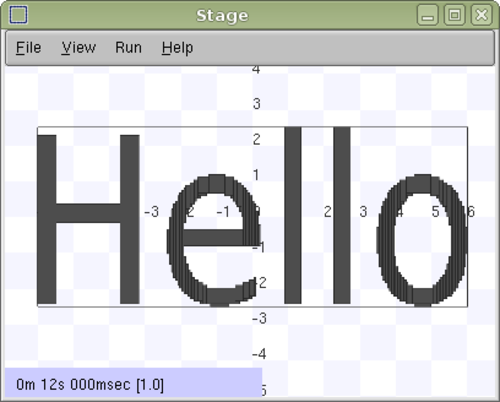 |
Figure 3.4: The first image is our “helloworld.png” bitmap, the second image is what Player/Stage interprets that bitmap as. The coloured areas are walls, the robot can move everywhere else.
A full list of model parameters and their descriptions can be found in the official Stage manual Most of the useful parameters have already been described here, however there are a few other types of model which are relevant to building simulations of robots, these will be described later in Section 3.2 - Building a Robot.
3.1.2 - Describing the Player/Stage Window
The worldfile also can be used to describe the simulation window that Player/Stage creates. Player/Stage will automatically make a window for the simulation if you don’t put any window details in the worldfile, however, it is often useful to put this information in anyway. This prevents a large simulation from being too big for the window, or to increase or decrease the size of the simulation.
Like a model, a window is an inbuilt, high-level entity with lots of parameters. Unlike models though, there can be only one window in a simulation and only a few of its parameters are really needed. The simulation window is described with the following syntax:
window
(
   # parameters...
)
The two most important parameters for the window are size and
scale.
size: This is the size the simulation window will be in pixels. You need to define both the width and height of the window using the following syntax:size [width height].scale: This is how many metres of the simulated environment each pixel shows. The bigger this number is, the smaller the simulation becomes. The optimum value for the scale is window_size/floorplan_size and it should be rounded downwards so the simulation is a little smaller than the window it’s in, some degree of trial and error is needed to get this right.
A full list of window parameters can be found in the Stage manual under “WorldGUI”
3.1.3 - Making a Basic Worldfile
We have already discussed the basics of worldfile building: models and the window. There are just a few more parameters to describe which don’t belong in either a model or a window description, these are optional though, and the defaults are pretty sensible.
interval_sim: This is how many simulated milliseconds there are between each update of the simulation window, the default is 100 milliseconds.interval_real: This is how many real milliseconds there are between each update of the simulation window. Balancing this parameter and theinterval_simparameter controls the speed of the simulation. Again, the default value is 100 milliseconds, both these interval parameter defaults are fairly sensible, so it’s not always necessary to redefine them.
The Stage manual contains a list of the high-level worldfile parameters
Finally, we are able to write a worldfile!
include "map.inc"

# configure the GUI window
window
(
   size [700.000 700.000]
   scale 41
)

# load an environment bitmap
floorplan
(
   bitmap "bitmaps/cave.png"
   size [15 15 0.5]
)
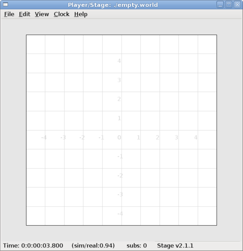
If we save the above code as empty.world (correcting any filepaths if necessary) we can run its corresponding empty.cfg file (see Section 3.1 - Empty World) to get the simulation shown in Figure 3.5.
| | | —————| |  | | Figure 3.5: Our Empty
World |
| | Figure 3.5: Our Empty
World |
3.2 - Building a Robot
In Player/Stage a robot is just a slightly advanced kind of model, all the parameters described in Models can still be applied.
3.2.1 - Sensors and Devices
There are six built-in kinds of model that help with building a robot,
they are used to define the sensors and actuators that the robot has.
These are associated with a set of model parameters which define by
which sensors the model can be detected (these are the _returns
mentioned earlier). Each of these built in models acts as an interface
(see Section 2.2 - Interfaces, Drivers, and
Devices) between the
simulation and Player. If your robot has one of these kinds of sensor on
it, then you need to use the relevant model to describe the sensor,
otherwise Stage and Player won’t be able to pass the data between each
other. It is possible to write your own interfaces, but the stuff
already included in Player/Stage should be sufficient for most people’s
needs. A full list of interfaces that Player supports can be found in
the Player
manual
although only the following are supported by the current distribution of
Stage (version 4.1.X). Unless otherwise stated, these models use the
Player interface that shares its name:
3.2.1.1 - camera
The camera model adds a camera to the robot model and allows your code to interact with the simulated camera. The camera parameters are as follows:
resolution [x y]: the resolution, in pixels, of the camera’s image.range [min max]: the minimum and maximum range that the camera can detectfov [x y]: the field of view of the camera in DEGREES.pantilt [pan tilt]: angle, in degrees, where the camera is looking. Pan is the left-right positioning. So for instance pantilt [20 10] points the camera 20 degrees left and 10 degrees down.
3.2.1.2 - blobfinder
The blobfinder simulates colour detection software that can be run on the image from the robot’s camera. It is not necessary to include a model of the camera in your description of the robot if you want to use a blobfinder, the blobfinder will work on its own.
In previous versions of Stage, there was a blob_return parameter to
determine if a blobfinder could detect an object. In Stage 4.1.1, this
does not seem to be the case. However, you can simply set an object to
be a color not listed in the colors[] list to make it invisible to
blobfinders.
The parameters for the blobfinder are described in the Stage manual, but the most useful ones are here:
colors_count <int>: the number of different colours the blobfinder can detectcolors [ ]: the names of the colours it can detect. This is given to the blobfinder definition in the form["black" "blue" "cyan"]. These colour names are from the built in X11 colour database rgb.txt. This is built in to Linux – the filergb.txtcan normally be found at /usr/share/X11/rgb.txt assuming it’s properly installed, or see Wikipedia for details.image [x y]: the size of the image from the camera, in pixels.range <float>: The maximum range that the camera can detect, in metres.fov <float>: field of view of the blobfinder in DEGREES. Unlike the camerafov, the blobfinderfovrespects theunit_anglecall as described in http://playerstage.sourceforge.net/wiki/Writing_configuration_files#Units. By default, the blobfinderfovis in DEGREES.
3.2.1.3 - fiducial
A fiducial is a fixed point in an image, so the fiducial
finder
simulates image processing software that locates fixed points in an
image. The fiducialfinder is able to locate objects in the simulation
whose fiducial_return parameter is set to true. Stage also allows
you to specify different types of fiducial using the fiducial_key
parameter of a model. This means that you can make the robots able to
tell the difference between different fiducials by what key they
transmit. The fiducial finder and the concept of fiducial_keys is
properly explained in the Stage manual. The fiducial sensors parameters
are:
range_min: The minimum range at which a fiducial can be detected, in metres.range_max: The maximum range at which a fiducial can be detected, in metres.range_max_id: The maximum range at which a fiducial’s key can be accurately identified. If a fiducial is closer thatrange_maxbut further away thanrange_max_idthen it detects that there is a fiducial but can’t identify it.fov: The field of view of the fiducial finder in DEGREES.
3.2.1.4 - ranger sensor
The ranger
sensor
simulates any kind of obstacle detection device (e.g. sonars, lasers, or
infrared sensors). These can locate models whose ranger_return is
non-negative. Using a ranger model you can define any number of ranger
sensors and apply them all to a single device. The parameters for the
sensor model and their inputs are described in the Stage manual, but
basically:
size [x y]: how big the sensors are.range [min max]: defines the minimum and maxium distances that can be sensed.fov deg: defines the field of view of the sensors in DEGREESsamples: this is only defined for a laser - it specifies ranger readings the sensor takes. The laser model behaves like a large number of rangers sensors all with the same x and y coordinates relative to the robot’s centre, each of these rangers has a slightly different yaw. The rangers are spaced so that there are samples number of rangers distributed evenly to give the laser’s field of view. So if the field of view is 180 and there are 180 samples the rangers are 1 apart.
3.2.1.5 - ranger device
A ranger
device is
comprised of ranger sensors. A laser is a special case of ranger sensor
which allows only one sensor, and has a very large field of view. For a
ranger device, you just provide a list of sensors which comprise this
device, typically resetting the pose for each. How to write the
[x y yaw] data is explained in Yaw Angles.
sensor_name (pose [x1 y1 z1 yaw1])
sensor_name (pose [x2 y2 z2 yaw2])
3.2.1.6 - gripper
The gripper model is a simulation of the gripper you get on a Pioneer robot. The Pioneer grippers looks like a big block on the front of the robot with two big sliders that close around an object. If you put a gripper on your robot model it means that your robot is able to pick up objects and move them around within the simulation. The online Stage manual says that grippers are deprecated in Stage 3.X.X, however this is not actually the case and grippers are very useful if you want your robot to be able to manipulate and move items. The parameters you can use to customise the gripper model are:
size [x y z]: The x and y dimensions of the gripper.pose [x y z yaw]: Where the gripper is placed on the robot, relative to the robot’s geometric centre. The pose parameter is decribed properly in Section 3.2.1 - Robot Sensors and Devices.
3.2.1.7 - position
The position
model
simulates the robot’s odometry, this is when the robot keeps track of
where it is by recording how many times its wheels spin and the angle it
turns. This robot model is the most important of all because it allows
the robot model to be embodied in the world, meaning it can collide with
anything which has its obstacle_return parameter set to true. The
position model uses the position2d interface, which is essential for
Player because it tells Player where the robot actually is in the world.
The most useful parameters of the position model are:
drive: Tells the odometry how the robot is driven. This is usually “diff” which means the robot is controlled by changing the speeds of the left and right wheels independently. Other possible values are “car” which means the robot uses a velocity and a steering angle, or “omni” which means it can control how it moves along the x and y axes of the simulation.localization: tells the model how it should record the odometry “odom” if the robot calculates it as it moves along or “gps” for the robot to have perfect knowledge about where it is in the simulation.odom_error [x y angle]: The amount of error that the robot will make in the odometry recordings.
3.2.2 - An Example Robot
To demonstrate how to build a model of a robot in Player/Stage we will build our own example. First we will describe the physical properties of the robot, such as size and shape. Then we will add sensors onto it so that it can interact with its environment.
3.2.2.1 - The Robot’s Body
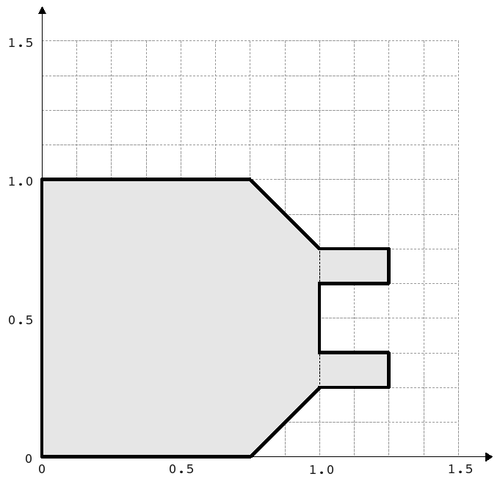
Let’s say we want to model a rubbish collecting robot called “Bigbob”.
The first thing we need to do is describe its basic shape, to do this
you need to know your robot’s dimensions in metres. Figure 3.6 shows the
basic shape of Bigbob drawn onto some cartesian coordinates, the
coordinates of the corners of the robot have been recorded. We can then
build this model using the block model parameter. In this example
we’re using blocks with the position model type but we could equally use
it with other model types.
| | | —————| | 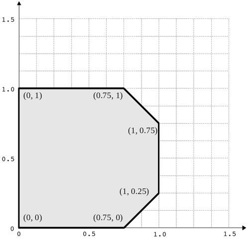 | | Figure 3.6: The basic
shape we want to make Bigbob, the units on the axes are in metres.|
| | Figure 3.6: The basic
shape we want to make Bigbob, the units on the axes are in metres.|
define bigbob position


      block
      (
            points 6
            point[0] [0.75 0]
            point[1] [1 0.25]
            point[2] [1 0.75]
            point[3] [0.75 1]
            point[4] [0 1]
            point[5] [0 0]
            z [0 1]
      )
)


bigbob
(
          name "bob1"
          pose [ 0 0 0 0]
          color "gray"
)
In the first line of this code we state that we are defining a
position model called bigbob. Next block declares that this
position model contains a block.
The following lines go on to describe the shape of the block;
points 6 says that the block has 6 corners and
point[number] [x y] gives the coordinates of each corner of the
polygon in turn. Finally, the z [height_from height_to] states how
tall the robot should be, the first parameter being a lower coordinate
in the z plane, and the second parameter being the upper coordinate in
the z plane. In this example we are saying that the block describing
Bigbob’s body is on the ground (i.e. its lower z coordinate is at 0)
and it is 1 metre tall. If I wanted it to be from 50cm off the ground to
1m then I could use z [0.5 1].
TRY IT OUT (Position Model)
In this example, you can see the basic shape in an empty environment.
3.2.2.2 - Adding Teeth
Now in the same way as we built the body we can add on some teeth for Bigbob to collect rubbish between. Figure 3.7 shows Bigbob with teeth plotted onto a cartesian grid:
 |
| Figure 3.7: The new shape of Bigbob. |
define bigbob position
(
      size [1.25 1 1]

      # the shape of Bigbob

      block
      (
            points 6
            point[5] [0 0]
            point[4] [0 1]
            point[3] [0.75 1]
            point[2] [1 0.75]
            point[1] [1 0.25]
            point[0] [0.75 0]
            z [0 1]
      )

      block
      (
            points 4
            point[3] [1 0.75]
            point[2] [1.25 0.75]
            point[1] [1.25 0.625]
            point[0] [1 0.625]
            z [0 0.5]
      )

      block
      (
            points 4
            point[3] [1 0.375]
            point[2] [1.25 0.375]
            point[1] [1.25 0.25]
            point[0] [1 0.25]
            z [0 0.5]
      )
)
To declare the size of the robot you use the size [x y z] parameter,
this will cause the polygon described to be scaled to fit into a box
which is x by y in size and z metres tall. The default size
is 0.4 x 0.4 x 1 m, so because the addition of rubbish-collecting teeth
made Bigbob longer, the size parameter was needed to stop Player/Stage
from making the robot smaller than it should be. In this way we could
have specified the polygon coordinates to be 4 times the distance apart
and then declared its size to be 1.25 x 1 x 1 metres, and we would
have got a robot the size we wanted. For a robot as large as Bigbob this
is not really important, but it could be useful when building models of
very small robots. It should be noted that it doesn’t actually matter
where in the cartesian coordinate system you place the polygon, instead
of starting at (0, 0) it could just as easily have started at
(-1000, 12345). With the block parameter we just describe the
shape of the robot, not its size or location in the map.
TRY IT OUT (BigBob with Teeth)
This example shows the more accurate rendering of Big Bob.
3.2.2.3 - Yaw Angles
You may have noticed that in Figures 3.6 and 3.7 Bigbob is facing to the
right of the grid. When you place any item in a Player/Stage simulation
they are, by default, facing to the right hand side of the simulation.
Figure 3.3 shows that the grids use a typical Cartesian coordinate
system, and so if you want to alter the direction an object in the
simulation is pointing (its “yaw”) any angles you give use the x-axis as
a reference, just like vectors in a Cartesian coordinate system (see
Figure 3.8) and so the default yaw is 0 degrees. This is also why in
Section 3.1 - Empty World the
gui_nose shows the map is facing to the right. Figure 3.9 shows a
few examples of robots with different yaws.
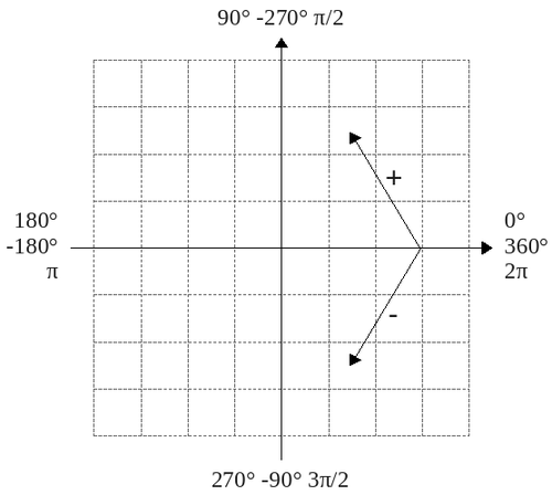 |
| Figure 3.8: A cartesian grid showing how angles are described. |
 |
| Figure 3.9: Starting from the top right robot and working anti-clockwise, the yaws of these robots are 0, 90, -45 and 200. |
By default, Player/Stage assumes the robot’s centre of rotation is at
its geometric centre based on what values are given to the robot’s
size parameter. Bigbob’s size is 1.25 x 1 x 1 so
Player/Stage will place its centre at (0.625, 0.5, 0.5), which means
that Bigbob’s wheels would be closer to its teeth. Instead let’s say
that Bigbob’s centre of rotation is in the middle of its main body
(shown in Figure 3.6 which puts the centre of rotation at
(0.5, 0.5, 0.5). To change this in robot model you use the
origin [x-offset y-offset z-offset] command:
define bigbob position
(
      # actual size
      size [1.25 1 1]
      # centre of rotation offset
      origin [0.125 0 0]

      # the shape of Bigbob
      block
            ...
            ...
            ...
)
TRY IT OUT (Different Origin)
Click on the robot, and it should hilight. You can drag bigbob around with the left (primay) mouse button. Click and hold down the right (secondary) mouse button, and move the mouse to rotate bigbob about the centre of the body, not the centre of the entire block.
3.2.2.4 - Drive
Finally we will specify the drive of Bigbob, this is a parameter of
the position model and has been described earlier.
define bigbob position
(
      # actual size
      size [1.25 1 1]
      # centre of rotation offset
      origin [0.125 0 0]

      # the shape of Bigbob
      block
            ...
            ...
            ...

      # positonal things
      drive "diff"
)
3.2.2.5 - The Robot’s Sensors
Now that Bigbob’s body has been built let’s move on to the sensors. We will put sonar and blobfinding sensors onto Bigbob so that it can detect walls and see coloured blobs it can interpret as rubbish to collect. We will also put a laser between Bigbob’s teeth so that it can detect when an item passes in between them.
Bigbob’s Sonar
We will start with the sonars. The first thing to do is to define a model for the sonar sensor that is going to be used on Bigbob:
define bigbobs_sonars sensor
(
      # parameters...
)
define bigbobs_ranger ranger
(
      # parameters...
)
Here we tell Player/Stage that we will define a type of sensor called bigbobs_sonars. Next, we’ll tell Player/Stage to use these sensors in a ranging device. Let’s put four sonars on Bigbob, one on the front of each tooth, and one on the front left and the front right corners of its body.
When building Bigbob’s body we were able to use any location on a
coordinate grid that we wanted and could declare our shape polygons to
be any distance apart we wanted so long as we resized the model with
size. In contrast, sensors - all sensors not just rangers - must be
positioned according to the robot’s origin and actual size. To work
out the distances in metres it helps to do a drawing of where the
sensors will go on the robot and their distances from the robot’s
origin. When we worked out the shape of Bigbob’s body we used its actual
size, so we can use the same drawings again to work out the distances of
the sensors from the origin as shown in Figure 3.10.
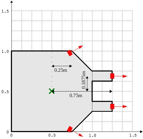 |
| Figure 3.10: The position of Bigbob’s sonars (in red) relative to its origin. The origin is marked with a cross, some of the distances from the origin to the sensors have been marked. The remaining distances can be done by inspection. |
First, we’ll define a single ranger (in this case sonar) sensor. To define the size, range and field of view of the sonars we just consult the sonar device’s datasheet.
define bigbobs_sonar sensor
(
    # define the size of each transducer [xsize ysize zsize] in meters
    size [0.01 0.05 0.01 ]
    # define the range bounds [min max]
    range [0.3 2.0]
    # define the angular field of view in degrees
    fov 10
    # define the color that ranges are drawn in the gui
    color_rgba [ 0 1 0 1 ]
)
Then, define how the sensors are placed into the ranger device. The process of working out where the sensors go relative to the origin of the robot is the most complicated part of describing the sensor.
define bigbobs_sonars ranger
(
  # one line for each sonar [xpos ypos zpos heading]
  bigbobs_sonar( pose [ 0.75 0.1875 0 0]) # fr left tooth
  bigbobs_sonar( pose [ 0.75 -0.1875 0 0]) # fr right tooth
  bigbobs_sonar( pose [ 0.25 0.5 0 30]) # left corner
  bigbobs_sonar( pose [ 0.25 -0.5 0 -30]) # right corner
)
TRY IT OUT (driving a robot)
This file includes everything described up till now.
This will start player in the background, then start a “remote control” (also in the background). You may need to move the playerv window out of the way to see the Stage window.
See the playerv documentation for details on playerv. For now, the “remote control” just makes the ranger sensor cones appear.
Bigbob’s Blobfinder
Now that Bigbob’s sonars are done we will attach a blobfinder:
define bigbobs_eyes blobfinder
(
      # parameters
)
Bigbob is a rubbish-collector so here we should tell it what colour of rubbish to look for. Let’s say that the intended application of Bigbob is in an orange juice factory and he picks up any stray oranges or juice cartons that fall on the floor. Oranges are orange, and juice cartons are (let’s say) dark blue so Bigbob’s blobfinder will look for these two colours:
define bigbobs_eyes blobfinder
(
      # number of colours to look for
      colors_count 2

      # which colours to look for
      colors ["orange" "DarkBlue"]
)
Then we define the properties of the camera, again these come from a datasheet:
define bigbobs_eyes blobfinder
(
      # number of colours to look for
      colors_count 2

      # which colours to look for
      colors ["orange" "DarkBlue"]

      # camera parameters
      image [160 120]   #resolution
      range 5.00        # m
      fov 60            # degrees
)
TRY IT OUT (blobfinder)
Similar to the previous example, playerv just makes the camera show
up in the PlayerViewer window.
Bigbob’s Laser
The last sensor that needs adding to Bigbob is the laser, which will be used to detect whenever a piece of rubbish has been collected, the laser’s location on the robot is shown in Figure 3.11. Following the same principles as for our previous sensor models we can create a description of this laser:
define bigbobs_laser sensor
(
      size [0.025 0.025 0.025]
      range [0 0.25]            # max = dist between teeth in m
      fov 20                    # does not need to be big
      color_rgba [ 1 0 0 0.5]
      samples 180               # number of ranges measured
)
define bigbobs_lasers ranger
(
      bigbobs_laser( pose [ 0.625 0.125 -0.975 270 ])
)
With this laser we’ve set its maximum range to be the distance between
teeth, and the field of view is arbitrarily set to 20 degrees. We have
calculated the laser’s pose in exactly the same way as the sonars
pose, by measuring the distance from the laser’s centre to the
robot’s origin (which we set with the origin parameter earlier). The
z coordinate of the pose parameter when describing parts of the robot
is relative to the very top of the robot. In this case the robot is 1
metre tall so we put the laser at -0.975 so that it is on the ground.
The laser’s yaw is set to 270 degrees so that it points across
Bigbob’s teeth. We also set the size of the laser to be 2.5cm cube so
that it doesn’t obstruct the gap between Bigbob’s teeth.
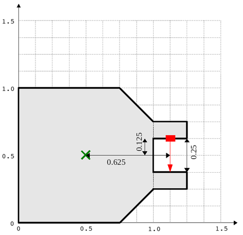 |
| Figure 3.11: The position of Bigbob’s laser (in red) and its distance, in metres, relative to its origin (marked with a cross). |
Now that we have a robot body and sensor models all we need to do is put
them together and place them in the world. To add the sensors to the
body we need to go back to the bigbob position model:
define bigbob position
(
      # actual size
      size [1.25 1 1]
      # centre of rotation offset
      origin [0.125 0 0]

      # the shape of Bigbob
      block
            ...
            ...
            ...

      # positonal things
      drive "diff"

      # sensors attached to bigbob
      bigbobs_sonars()
      bigbobs_eyes()
      bigbobs_laser()
)
The extra line bigbobs_sonars() adds the sonar model called
bigbobs_sonars() onto the bigbob model, likewise for
bigbobs_eyes() and bigbobs_laser().
At this point it’s worthwhile to copy this into a .inc file, so that the model could be used again in other simulations or worlds. This file can also be found in the example code in /Ch5.3/bigbob.inc
To put our Bigbob model into our empty world (see Section 3.1.3 -
Making a Basic Worldfile) we need to
add the robot to our worldfile empty.world:
include "map.inc"
include "bigbob.inc"

# size of the whole simulation
size [15 15]


# configure the GUI window
window
(
      size [ 700.000 700.000 ]
      scale 35
)


# load an environment bitmap
floorplan
(
      bitmap "bitmaps/cave.png"
      size [15 15 0.5]
)

bigbob
(
      name "bob1"
      pose [-5 -6 0 45]
      color "green"
)
Here we’ve put all the stuff that describes Bigbob into a .inc file
bigbob.inc, and when we include this, all the code from the .inc
file is inserted into the .world file. The section here is where we put
a version of the bigbob model into our world:
bigbob
(
      name "bob1"
      pose [-5 -6 0 45]
      color "green"
)
Bigbob is a model description, by not including any define stuff in
the top line there it means that we are making an instantiation of that
model, with the name bob1. Using an object-oriented programming
analogy, bigbob is our class, and bob1 is our object of class
bigbob. The pose [x y yaw] parameter works in the same way as
spose [x y yaw] does. The only differences are that the coordinates
use the centre of the simulation as a reference point and pose lets
us specify the initial position and heading of the entire bob1
model, not just one sensor within that model.
Finally we specify what colour bob1 should be, by default this is
red. The pose and color parameters could have been specified in
our bigbob model but by leaving them out it allows us to vary the colour
and position of the robots for each different robot of type bigbob,
so we could declare multiple robots which are the same size, shape and
have the same sensors, but are rendered by Player/Stage in different
colours and are initialised at different points in the map.
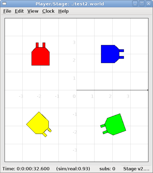
When we run the new bigbob6.world with Player/Stage we see our
Bigbob robot is occupying the world, as shown in Figure 3.12.
| | | —————| | 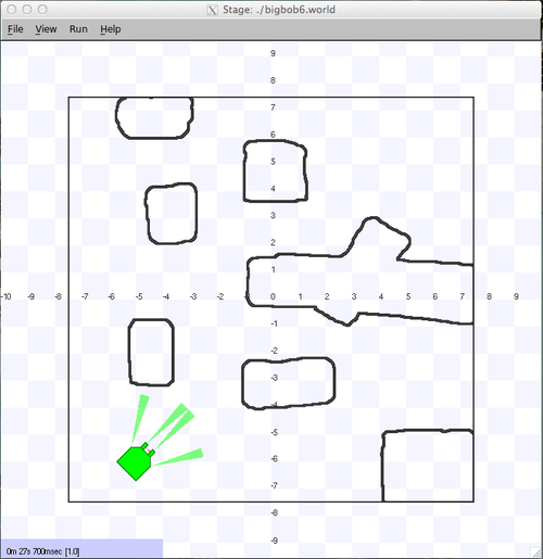 | | Figure 3.12: Our bob1
robot placed in the simple world, showing the range and field of view of
all of the ranger sensors. |
| | Figure 3.12: Our bob1
robot placed in the simple world, showing the range and field of view of
all of the ranger sensors. |
TRY IT OUT (Bigbob in environment)
This should show you Figure 3.12
You may wish to zoom in on the teeth to see the tooth laser.
3.2.3 - Building Other Stuff
We established in Section 3.2.2 - An Example Robot that Bigbob works in a orange juice factory collecting oranges and juice cartons. Now we need to build models to represent the oranges and juice cartons so that Bigbob can interact with things.
oranges
We’ll start by building a model of an orange:
define orange model
(
      # parameters...
)
The first thing to define is the shape of the orange. The block
parameter is one way of doing this, which we can use to build a blocky
approximation of a circle. An alternative to this is to use bitmap
which we previously saw being used to create a map. What the bitmap
command actually does is take in a picture, and turn it into a series of
blocks which are connected together to make a model the same shape as
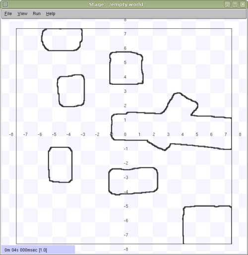
the picture, as illustrated in Figure 3.13 for an alien bitmap.
 |
 |
Figure 3.13: The left image is the original picture, the right image is its Stage interpretation.
In our code, we don’t want an alien, we want a simple circular shape (see Figure 3.14), so we’ll point to a circular bitmap.
 |
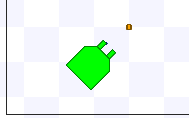 |
Figure 3.14: The orange model rendered in the same Stage window as Bigbob.
define orange model
(
      bitmap "bitmaps/circle.png"
      size [0.15 0.15 0.15]
      color "orange"
)
In this bit of code we describe a model called orange which uses a
bitmap to define its shape and represents an object which is 15cm x
15cm x 15cm and is coloured orange. Figure 3.14 shows our orange
model next to Bigbob.
Juice Cartons
Building a juice carton model is similarly quite easy:
define carton model
(
      # a carton is retangular
      # so make a square shape and use size[]
      block
      (
            points 4
            point[0] [1 0]
            point[1] [1 1]
            point[2] [0 1]
            point[3] [0 0]
            z [0 1]
      )

      # average litre carton size is ~ 20cm x 10cm x 5cm ish
      size [0.1 0.2 0.2]

      color "DarkBlue"
)
We can use the block command since juice cartons are boxy, with boxy
things it’s slightly easier to describe the shape with block than
drawing a bitmap and using that. In the above code I used block to
describe a metre cube (since that’s something that can be done pretty
easily without needing to draw a carton on a grid) and then resized it
to the size I wanted using size.
Putting objects into the world
Now that we have described basic orange and carton models it’s
time to put some oranges and cartons into the simulation. This is done
in the same way as our example robot was put into the world:
orange
(
      name "orange1"
      pose [-2 -5 0 0]
)

carton
(
      name "carton1"
      pose [-3 -5 0 0]
)
We created models of oranges and cartons, and now we are declaring that
there will be an instance of these models (called orange1 and
carton1 respectively) at the given positions. Unlike with the robot,
we declared the color of the models in the description so we don’t
need to do that here. If we did have different colours for each orange
or carton then it would mess up the blobfinding on Bigbob because the
robot is only searching for orange and dark blue. At this point it would
be useful if we could have more than just one orange or carton in the
world (Bigbob would not be very busy if there wasn’t much to pick up),
it turns out that this is also pretty easy:
orange(name "orange1" pose [-1 -5 0 0])
orange(name "orange2" pose [-2 -5 0 0])
orange(name "orange3" pose [-3 -5 0 0])
orange(name "orange4" pose [-4 -5 0 0])

carton(name "carton1" pose [-2 -4 0 0])
carton(name "carton2" pose [-2 -3 0 0])
carton(name "carton3" pose [-2 -2 0 0])
carton(name "carton4" pose [-2 -1 0 0])
Up until now we have been describing models with each parameter on a new
line, this is just a way of making it more readable for the programmer
– especially if there are a lot of parameters. If there are only a few
parameters or you want to be able to comment it out easily, it can all
be put onto one line. Here we declare that there will be four orange
models in the simulation with the names orange1 to orange4, we
also need to specify different poses for the models so they aren’t all
on top of each other. Properties that the orange models have in common
(such as shape, colour or size) should all be in the model definition.
TRY IT OUT (full worldfile)
This should show you Figure 3.15.
The full worldfile is at <source_code>/Ch3/bigbob7.world, this
includes the orange and carton models as well as the code for putting
them in the simulation. Figure 3.15 shows the populated Player/Stage
simulation.
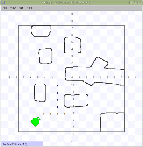 |
| Figure 3.15: The Bigbob robot placed in the simulation along with junk for it to pick up. |
img